Is intelligence really normally distributed?

a left-tailed bell curve

Few, if any, human traits correspond to a true normal distribution.

The mean height of men globally is about 171cm, with a standard deviation of 7.6 cm. If height followed a normal distribution, it would be close to impossible for there to be people with heights 6.2 standard deviations above the mean, yet there are plenty of people who are taller than 218cm (7’2’’). Even if the average global height were equal to that of European-descended men (180cm), the tallest people in the world would be predicted to be about 227cm (7’6’’). This is empirically not supported either — there are five people who are 244cm or taller who live today.

Disorders like gigantism cause people to grow to heights beyond what are expected from the sum of regular additive genetic factors and environments, and the same holds for dwarfism.

Another violation of normality that is seen in statistical distributons is skewness, where the tail of the distribution is skewed towards one side of the distribution. In the case of BMI, the tail is more prominent at the right side of the distribution, while for age at death the opposite is the case. This is probably due to the fact that there are more ways to shift to one side of the distribution than the other: there are many ways to die, but only one to live — not die.

Violations of normality can also arise from multiplicative distributions. If a trait is influenced by many additive genetic and environmental effects, the distribution will be close to normal, while the distribution of a trait that is influenced by many multiplicative effects will follow a log-normal distribution, which is a distribution which, when log-transformed, follows a normal distribution. In 97-99% of the population, income follows a log-transformed distribution.

As humans have been selected for intelligence for at least 10,000 years, genetic variants that have strong effects on intelligence will have largely reached fixation within humans. This means that when mutations cause these alleles to change, they will almost always result in reductions to intelligence. Empirically, all rare variants associated with education tend to have large negative effects on the trait.

from here

If this is the case, then mutations should shift the distribution of intelligence towards the left, similar to the way dwarfism causes lots of outliers in terms of height.

The best dataset to test this theory out is the Project Talent, a study of American highschoolers, due to the fact that it has a many subtests (59, including the iffy ones) and tested a large number of individuals (~370,000). People that were either under 14 or over 18 were removed to avoid selection biasing the age effects, and the sample was subset to White, non-Jewish men with data on their ages. This left 68,000 individuals, which is more than enough to test for the existence of normality.

To calculate levels of intelligence, the first unrotated principal component was extracted out of the 59 tests, with age partialled out afterwards. The distribution of scores is as follows:

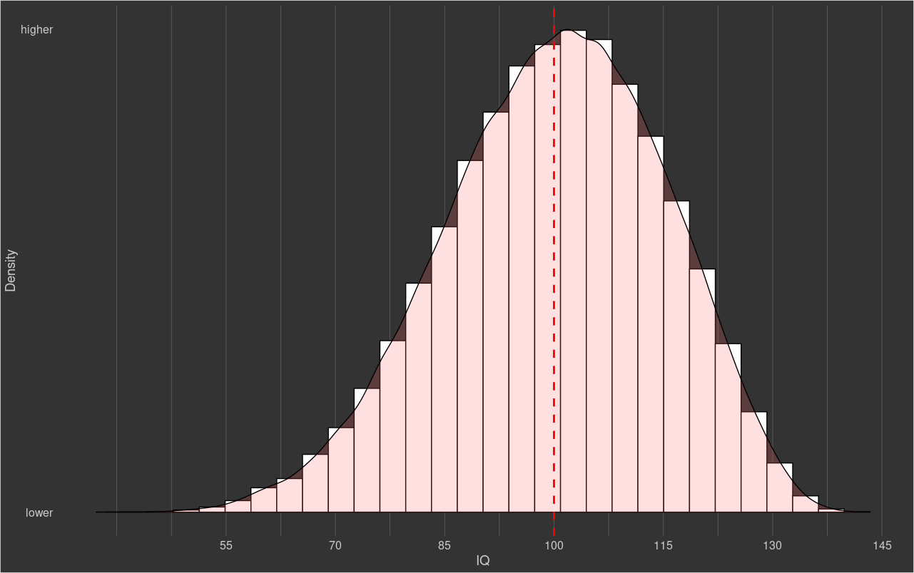
The scores had a skew and kurtosis¹ of -0.26, indicating that the distribution was a left-tailed distribution with a relative lack of outliers. The standard errors of these estimates are extremely low: 0.01 for skewness and 0.02 for kurtosis, so the estimates would pass any conventional significance testing.

Kurtosis in this article is real kurtosis - 3 for the sake of simplicity. This makes it so that negative kurtosis is less outliers, and positive kurtosis is more outliers.

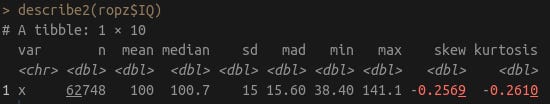
The minimum score was 38.4, while the maximum score was 141.1. If these scores followed a normal distribution, it would be expected that the top score would be about 160, a score 50% more extreme than the one that was actually observed.

A nice vindication of the theory, but it would be prudent to test whether this an artefact of violations in normality observed within the individual subtests. The idea being that, perhaps the scores have a skewed distribution to the left because subtests that form the battery are as well.

To do this, the subtests were transformed to a rank-ordered distribution which was then converted to a normal distribution. That caused the subtests to look more normal, but all of them had a kurtosis of ~0.2 and skewness of ~-0.2. To fix that, a Yeo-Johnson transformation was applied, though many subtests were still not normally distributed. The van der Waerden transformation was applied to this transformed data after the first transformation, and now 13 subtests finally had a skewness and kurtosis of between -0.1 and 0.1. A general score was calculated from these tests, age was controlled for, and finally, the distribution was plotted.

Roughly the same distribution, but with less kurtosis.

There is no guarantee that this finding applies outside of this dataset, so I checked three other datasets that had more than 9 subtests of intelligence (earlier I had ommitted the names, but they are the NLSY79, NLSY97, and ABCD datasets²). Even after the subtests were deliberately manipulated to fit a normal distribution, as was done before, in all 3 cases, the factor scores had a skewness of between -0.2 and -0.3.

If the individual subtests cannot be blamed for the artefact, then that implies that the true distribution of intelligence is indeed left-tailed and possibly deficient in outliers as well. Which is interesting — this supports the theory that Spearman’s Law of Diminishing Returns is an artefact of intelligence not having a normal distribution. This does not necessarily imply that general intelligence has the same effect on cognitive performance at each part of the distribution, just that Spearman’s Law cannot be cited to state this is the case.

Edit — Inquisitive bird mentions Johnson et al (2008) who also find evidence for a non-normal distribution within the Scottish Mental Surveys of 1932 and 1947, both of which tested most of Scotland’s 11 year olds:

The most obvious departure was that neither distribution was symmetric: in each survey, more scores were below the peak of the distribution than above it, indicating negative skewness. Skewness was -.211 and -.347 in SMS32 and SMS47, respectively. These skewness values do not sound excessive by common standards, but they were highly statistically significant in these large samples. If we want to understand the distribution of general intelligence at the level of the population, these skewness results matter.

Part 2

1. Kurtosis: how many outliers the distribution has relative to a normal bell curve.

Skewness: how the distribution skews relative to a normal bell curve.

2. I deleted the ABCD code a while ago, but this was the start of the code:

kitty <- readRDS('data/nda3.0.Rds')

kitty$card <- kitty$nihtbx_cardsort_uncorrected
kitty$voc <- kitty$nihtbx_picvocab_theta
kitty$flank <- kitty$nihtbx_flanker_uncorrected
kitty$mem <- kitty$nihtbx_list_uncorrected
kitty$sdmemory <- kitty$pea_ravlt_sd_trial_vi_tc
kitty$ldmemory <- kitty$pea_ravlt_ld_trial_vii_tc
kitty$read <- kitty$nihtbx_reading_theta
kitty$oralread <- as.numeric(kitty$nihtbx_reading_theta)
kitty$speed <- kitty$nihtbx_pattern_uncorrected
kitty$seqmem <- kitty$nihtbx_picture_theta
kitty$matrix <- kitty$pea_wiscv_trs

cor(kitty %>% select(card, voc, flank, mem, read, oralread, speed, seqmem, matrix, ldmemory, sdmemory), use='pairwise.complete.obs')

fa(kitty %>% select(card, voc, flank, mem, read, oralread, speed, seqmem, matrix, ldmemory, sdmemory))


kitty$g <- getpc(kitty %>% select(card, voc, flank, mem, read, oralread, speed, seqmem, matrix, ldmemory, sdmemory), dofa=F, fillmissing=F, normalizeit = T)

Code for NLSY97:

library(rms)
subtestlist <- c('GS', 'AR', 'WK', 'PC', 'NO', 'CS', 'AI', 'SI', 'MK', 'MC', 'EI', 'AO')
new_data$GS = NA
new_data$AR = NA
new_data$WK = NA
new_data$PC = NA
new_data$NO = NA
new_data$CS = NA
new_data$AI = NA
new_data$SI = NA
new_data$MK = NA
new_data$MC = NA
new_data$EI = NA
new_data$AO = NA

new_data$testday = new_data$R9708601*1/12+new_data$R9708602

new_data$testday[is.na(new_data$testday)] <- 1997.661

new_data$bdate = new_data$R0536402 + new_data$R0536401*1/12

new_data$age = new_data$testday-new_data$bdate

new_data$ageat = 1997 - new_data$bdate

j = 0
for(stest in subtestlist) {
  posstring = paste("R", 9705200+j*100, sep="")
  negstring = paste("R", 9706400+j*100, sep="")
  stcolumnindex = getcolindex(stest, new_data)
  negcolumnindex = getcolindex(negstring, new_data)
  poscolumnindex = getcolindex(posstring, new_data)
  new_data[, stcolumnindex] = as.numeric(pmax(new_data[, negcolumnindex]*-1, new_data[, poscolumnindex], na.rm=TRUE))
  new_data[, stcolumnindex] = normalise(new_data[, stcolumnindex])
  new_data[, stcolumnindex][!is.na(new_data[, stcolumnindex])] <- agecorrect(stest, 'ageat', normalizeit=T, datafr=new_data, splinex=4)
  j = j+1
}

new_data$race <- ""
new_data$race[new_data$white==1] <- 'White'
new_data$race[new_data$jew==1] <- 'Jewish'
new_data$race[new_data$amerind==1] <- 'Amerindian'
new_data$race[new_data$hispanic==1] <- 'Hispanic'
new_data$race[new_data$black==1] <- 'Black'

###############
whiteman <- new_data %>% filter(Female==0 & race=='White')

for(abi in subtestlist) {
  print(abi)
  whiteman$totest <- whiteman[[abi]]
  
  whiteman$rank <- ranker(whiteman$totest)
  lengthcol <- nrow(whiteman %>% filter(!is.na(abi)))
  whiteman$normrank <- -qnorm(whiteman$rank/(lengthcol+1))
  whiteman[[abi]] <- whiteman$normrank
}

for (col in subtestlist) {
  whiteman[[col]] <- yeojohnson(whiteman[[col]])$x.t
}
for (col in subtestlist) {
  whiteman[[col]] <- bestNormalize::orderNorm(whiteman[[col]])$x.t
}

upset <- describe2(whiteman %>% select(subtestlist))
whiteman$g = getpc(whiteman %>% select(subtestlist), dofa=F, fillmissing=F, normalizeit=T)
whiteman$IQ = whiteman$g*15+100

GG_denhist(whiteman, 'IQ')
describe2(whiteman$IQ)

Code for NLSY79:

distvec <- c(0.005, 0.01, 0.05, 0.1, 0.25, 0.5, 0.75, 0.9, 0.95, 0.99, 0.995)
##############
#race and g

iqtests <- c('R0615000', 'R0615100', 'R0615200', 'R0615300', 'R0615400', 'R0615500', 'R0615600', 'R0615700', 'R0615800', 'R0615900')
new_data$race = ""
new_data$race[new_data$R0214700==3] = 'White'
new_data$race[new_data$R0010310==8] = 'Jewish'
new_data$race[new_data$R0214700==2] = 'Black'
new_data$race[new_data$R0214700==1] = 'Hispanic'
new_data$race[new_data$R0010310==107] = 'Subindian'
new_data$R0214800

whiteman <- new_data %>% filter(R0214800==1 & race=='White')

for(abi in iqtests) {
  print(abi)
  whiteman$totest <- whiteman[[abi]]
  
  whiteman$rank <- ranker(whiteman$totest)
  lengthcol <- nrow(whiteman %>% filter(!is.na(abi)))
  whiteman$normrank <- -qnorm(whiteman$rank/(lengthcol+1))
  whiteman[[abi]] <- whiteman$normrank
}

for (col in iqtests) {
  whiteman[[col]] <- yeojohnson(whiteman[[col]])$x.t
}
for (col in iqtests) {
  whiteman[[col]] <- bestNormalize::orderNorm(whiteman[[col]])$x.t
}

for (col in iqtests) {
  whiteman[[col]] <- yeojohnson(whiteman[[col]])$x.t
  #whiteman[[col]] <- whiteman[[col]]^1.2
}
upset <- describe2(whiteman %>% select(iqtests))
upset

whiteman$g = getpc(whiteman %>% select(iqtests), dofa=F, fillmissing=F, normalizeit=T)
whiteman$IQ = whiteman$g*15+100

GG_denhist(whiteman, 'IQ')
describe2(whiteman$IQ)