Conservative breeding revolution: not happening

Not in a hundred years

The contrarian attractor field has begun discussing fertility differences between conservatives and liberals, prompted by this chart:

dramatic difference

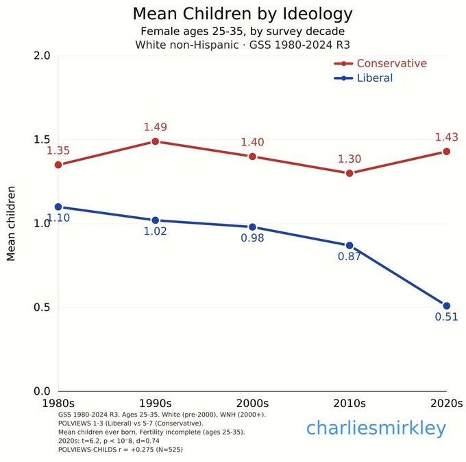
The idea of conservatives eventually outbreeding liberals is old, popularised by Kaufmann indirectly and then the HBD community. Somebody tried projecting the conservative share of the electorate using that data:

from here

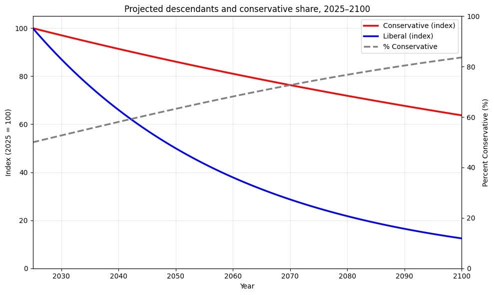
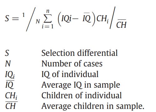
The right way to do this is to use the breeder’s equation, which estimates phenotypic changes in populations based on the relationship between a trait and surviving offspring. This is the formula:

ΔZ denotes the phenotypic change in the population, h^2 denotes the heritability, S denotes the relationship between fertility and the phenotype (selection differential)

The hard part comes with projecting what the relationship will be in the future. What I decided to do was weigh recent years more heavily when calculating the selection differential. If the strong fertility difference between conservatives/liberals persists in the future, then this will be an underestimate; if it regresses to the mean, then it will be an accurate estimate. I used the same measure of political views they did: self-reported placement on a 1-7 conservative/liberal scale.

I controlled political beliefs for age, year, race, and sex effects.

I got 0.07 standard deviations per generation¹, 0.035 when taking into account the 45% heritability of political views.

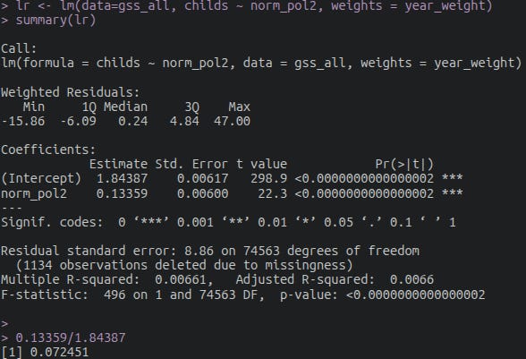
That equates to 0.1 standard deviations per century. That’s equivalent to going from the 50th to 54th percentile of conservatism. About an order of magnitude weaker than the original chart showed.

So, yeah.

Asides

Projecting using only post 2020 data

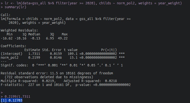
The change went from 0.035 SD per generation to 0.06 SD.

Better rendition — the correlation between fertility and conservatism has been steadily increasing with every cohort since 1920:

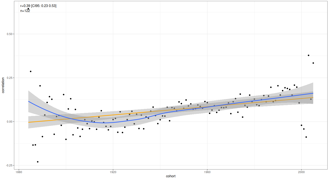
The average person in the GSS dataset was born in 1951, the correlation between conservatism and fertility at this time was about 0.08. In zoomers, it’s about 0.2. If we generously assume that means that the breeder’s equation underestimates the change by a factor of 0.2/0.08, then the projected change per century is 0.21 standard deviations².

Even then, a person in 2126 is projected to be at the 59th percentile of conservatism of a person in 2026.

Measurement error

Survey responses for measurable data (e.g. height, weight) tend to be very accurate, with correlations between reported and measured data being close to 1. There’s no reason to think number of children is different.

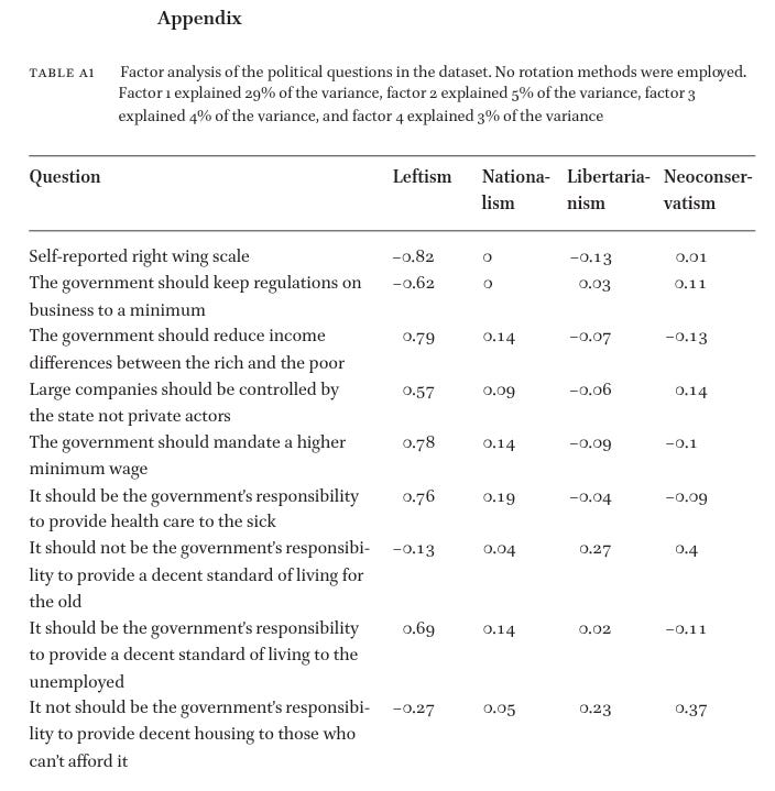
Regarding self-reported political views on a scale — they load at 0.82 on the primary factor of political views (right vs left):

from here

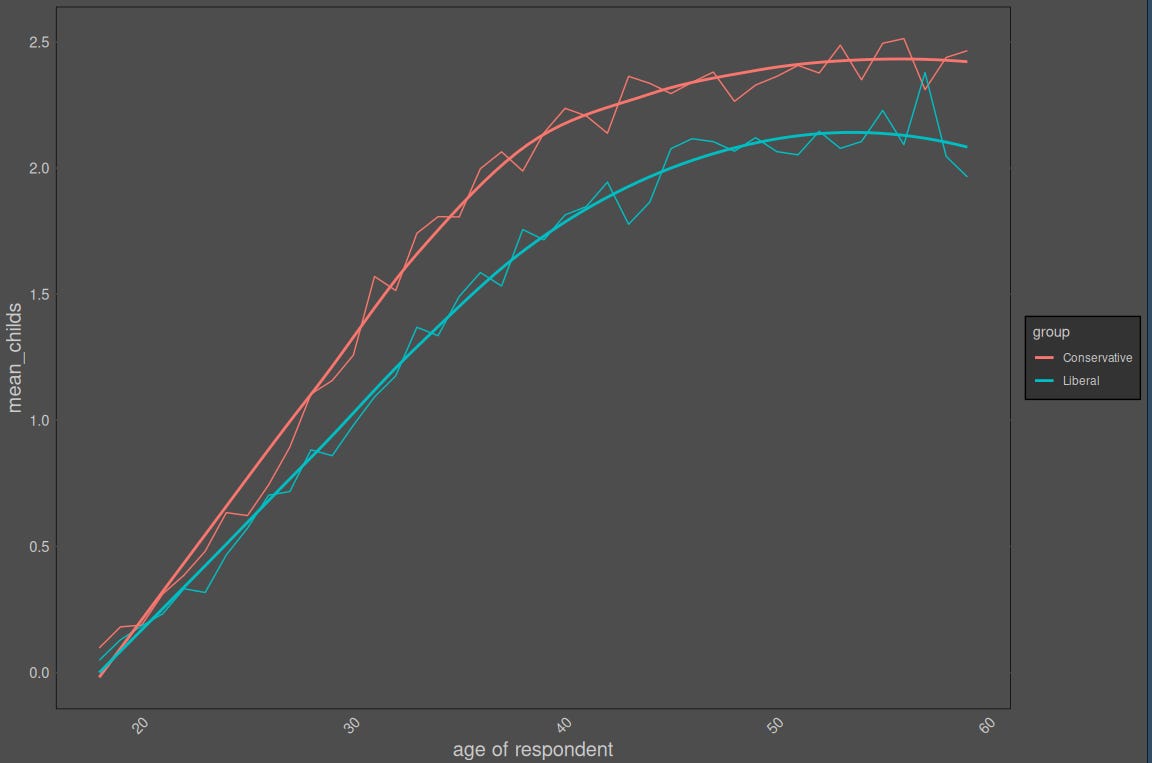
Differential ferility/age gradients by political views

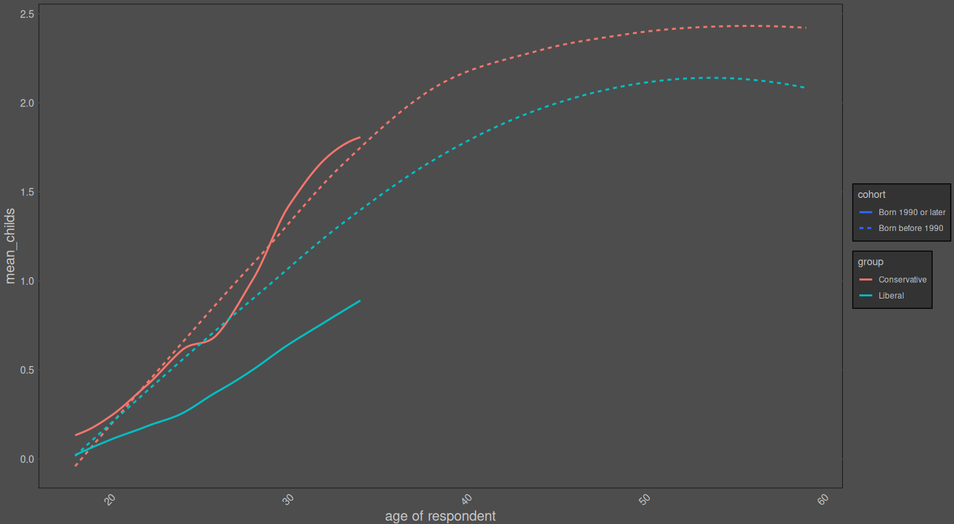
Nope. Conservatives and liberals seem to have kids at the same ages, just at different rates.

Better chart:

Heritability not 45%

Political beliefs are not genetic. The Communist manifesto was not coded into Marx’s genes. That said, there are personality traits and physiologies that are genetically influenced, which then can influence people’s political beliefs.

If one analyses twin/family correlations, a heritability of 40-50% fits the data well.

from here

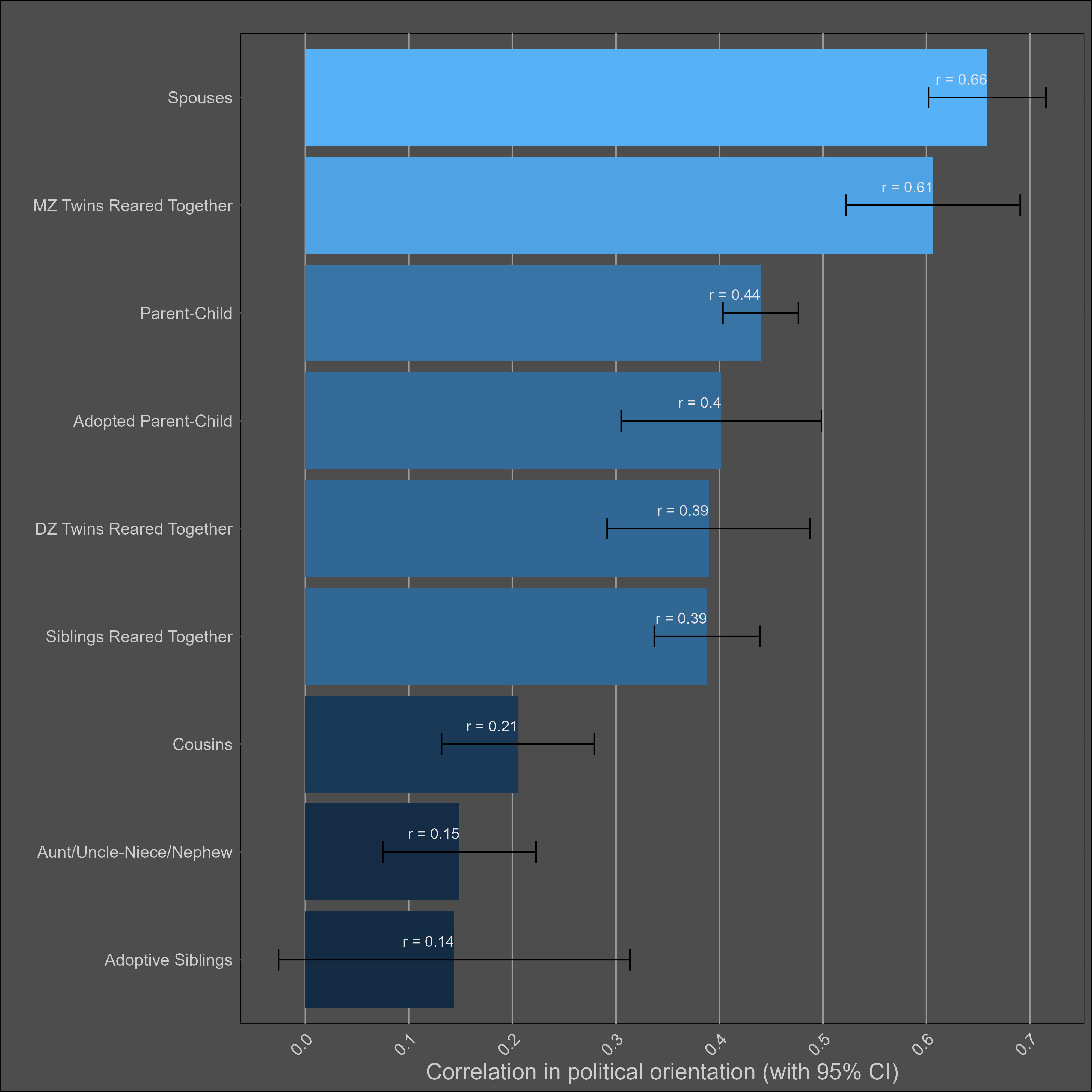
Many have asked that, if political beliefs are genetic, then why haven’t zoomers gotten more conservative? This is one of the many genotypic ~ phenotypic paradoxes, where one would expect the population to change one way based on the genes, but they actually changed in the opposite direction. It’s an artefact of the environment changing across time.

Causality

I’ve seen people make the argument that children cause people to be conservative more than being conservative causes fertility. It’s not intuitively impossible, but it’s a bad explanation for why the fertility difference between conservatives/liberals haas increased with time. It also doesn’t explain why conservatives want more children than liberals before they even have them.

1. Formula for selection differential (modified for IQ):

Short code:

install.packages('drat')
remotes::install_github("kjhealy/gssr")
library(gssr)
data(gss_all)

selection_differential <- function(iq, kid) {
  d <- data.frame(iq, kid)
  d <- na.omit(d)
  d$iq <- normalise(d$iq)
  parameter <- 0
  estimate <- 0
  daf <- data.frame(parameter, estimate)
  daf$parameter <- nrow(d)-2
  daf$estimate <- 1/nrow(d)*sum((d$iq-mean(d$iq, na.rm=T))*d$kid, na.rm=T)/mean(d$kid, na.rm=T)
  return(daf)
}

selection_differential_regression <- function(iq, kid) {
  d <- data.frame(iq, kid)
  d <- na.omit(d)
  d$iq <- normalise(d$iq)
  parameter <- 0
  estimate <- 0
  daf <- data.frame(parameter, estimate)
  
  if(nrow(d) > 0) {
    lr <- lm(data=d, kid ~ iq)
    
    daf$parameter <- nrow(d)-2
    daf$estimate <- lr$coefficients[2]/lr$coefficients[1]
  }
  else {
    daf$parameter <- NA
    daf$estimate <- NA
  }
  
  
  return(daf)
}

############################################

> gss_all$year_weight <- gss_all$year - min(gss_all$year, na.rm=T) + 1
> 
> describe2(gss_all$sex)
# A tibble: 1 × 10
  var       n   mean median      sd   mad   min   max     skew kurtosis
  <chr> <dbl>  <dbl>  <dbl>   <dbl> <dbl> <dbl> <dbl>    <dbl>    <dbl>
1 x     75568 1.5574      2 0.49669     0     1     2 -0.23125  -1.9465
> 
> gss_all$rcas <- 'White'
> gss_all$rcas[gss_all$race==1] <- 'White'
> gss_all$rcas[gss_all$relig==3] <- 'Jewish'
> gss_all$rcas[gss_all$race==3] <- 'Other'
> gss_all$rcas[gss_all$race==2] <- 'Black'
> gss_all$rcas[gss_all$hispanic>1] <- 'Hispanic'
> 
> gss_all$norm_pol <- normalise(gss_all$polviews)
> 
> lr <- lm(data=gss_all, norm_pol ~ rcs(year, 5) + rcs(age, 5) + rcas + sex)
> summary(lr)

Call:
lm(formula = norm_pol ~ rcs(year, 5) + rcs(age, 5) + rcas + sex, 
    data = gss_all)

Residuals:
    Min      1Q  Median      3Q     Max 
-2.5315 -0.6405 -0.0352  0.6406  2.7766 

Coefficients:
                     Estimate Std. Error t value             Pr(>|t|)    
(Intercept)         -17.92111    4.23071   -4.24    0.000022789504732 ***
rcs(year, 5)year      0.00881    0.00214    4.12    0.000038043096970 ***
rcs(year, 5)year'    -0.02203    0.01069   -2.06                0.039 *  
rcs(year, 5)year''    0.03622    0.03612    1.00                0.316    
rcs(year, 5)year'''  -0.00622    0.04704   -0.13                0.895    
rcs(age, 5)age        0.00985    0.00181    5.44    0.000000053434210 ***
rcs(age, 5)age'       0.00284    0.01574    0.18                0.857    
rcs(age, 5)age''     -0.02919    0.04344   -0.67                0.502    
rcs(age, 5)age'''     0.04268    0.04180    1.02                0.307    
rcasHispanic          0.14476    0.01927    7.51    0.000000000000059 ***
rcasJewish           -0.34026    0.03050  -11.15 < 0.0000000000000002 ***
rcasOther             0.04799    0.02271    2.11                0.035 *  
rcasWhite             0.22806    0.01151   19.82 < 0.0000000000000002 ***
sex                  -0.07173    0.00778   -9.22 < 0.0000000000000002 ***
---
Signif. codes:  0 ‘***’ 0.001 ‘**’ 0.01 ‘*’ 0.05 ‘.’ 0.1 ‘ ’ 1

Residual standard error: 0.985 on 65081 degrees of freedom
  (10604 observations deleted due to missingness)
Multiple R-squared:  0.029,	Adjusted R-squared:  0.0288 
F-statistic:  150 on 13 and 65081 DF,  p-value: <0.0000000000000002

> 
> gss_all$norm_pol2[!is.na(gss_all$age) & !is.na(gss_all$rcas) & !is.na(gss_all$sex) & !is.na(gss_all$age) & !is.na(gss_all$norm_pol)] <- lr$residuals
> gss_all$norm_pol2 <- normalise(gss_all$norm_pol2)
> 
> lr <- lm(data=gss_all, childs ~ norm_pol2, weights = year_weight)
> summary(lr)

Call:
lm(formula = childs ~ norm_pol2, data = gss_all, weights = year_weight)

Weighted Residuals:
   Min     1Q Median     3Q    Max 
-15.86  -6.09   0.24   4.84  47.02 

Coefficients:
            Estimate Std. Error t value            Pr(>|t|)    
(Intercept)  1.84386    0.00617   298.9 <0.0000000000000002 ***
norm_pol2    0.13347    0.00600    22.2 <0.0000000000000002 ***
---
Signif. codes:  0 ‘***’ 0.001 ‘**’ 0.01 ‘*’ 0.05 ‘.’ 0.1 ‘ ’ 1

Residual standard error: 8.86 on 74563 degrees of freedom
  (1134 observations deleted due to missingness)
Multiple R-squared:  0.00659,	Adjusted R-squared:  0.00658 
F-statistic:  495 on 1 and 74563 DF,  p-value: <0.0000000000000002

> 
> lr <- lm(data=gss_all, childs ~ norm_pol2)
> summary(lr)

Call:
lm(formula = childs ~ norm_pol2, data = gss_all)

Residuals:
   Min     1Q Median     3Q    Max 
-2.192 -1.754  0.019  1.069  6.352 

Coefficients:
            Estimate Std. Error t value            Pr(>|t|)    
(Intercept)  1.91171    0.00642   297.7 <0.0000000000000002 ***
norm_pol2    0.10495    0.00642    16.3 <0.0000000000000002 ***
---
Signif. codes:  0 ‘***’ 0.001 ‘**’ 0.01 ‘*’ 0.05 ‘.’ 0.1 ‘ ’ 1

Residual standard error: 1.75 on 74563 degrees of freedom
  (1134 observations deleted due to missingness)
Multiple R-squared:  0.00357,	Adjusted R-squared:  0.00355 
F-statistic:  267 on 1 and 74563 DF,  p-value: <0.0000000000000002

> 0.2/0.08*0.05504*0.45*100/30
[1] 0.2064
> 
> 0.10522/1.91171
[1] 0.05504
> 
> GG_scatter(gss_all, 'norm_pol2', 'norm_pol')
`geom_smooth()` using formula = 'y ~ x'
> 
> 0.13359/1.84387
[1] 0.072451
> 
> lr <- lm(data=gss_all, childs ~ norm_pol)
> summary(lr)

Call:
lm(formula = childs ~ norm_pol, data = gss_all)

Residuals:
   Min     1Q Median     3Q    Max 
 -2.27  -1.59   0.00   1.00   6.55 

Coefficients:
            Estimate Std. Error t value            Pr(>|t|)    
(Intercept)   1.8754     0.0067   280.0 <0.0000000000000002 ***
norm_pol      0.1921     0.0067    28.7 <0.0000000000000002 ***
---
Signif. codes:  0 ‘***’ 0.001 ‘**’ 0.01 ‘*’ 0.05 ‘.’ 0.1 ‘ ’ 1

Residual standard error: 1.72 on 65654 degrees of freedom
  (10043 observations deleted due to missingness)
Multiple R-squared:  0.0124,	Adjusted R-squared:  0.0124 
F-statistic:  823 on 1 and 65654 DF,  p-value: <0.0000000000000002

> 
> 
> selection_differential(iq=gss_all$norm_pol, kid=gss_all$childs)
  parameter estimate
1     65654  0.10244
> selection_differential_regression(iq=gss_all$norm_pol, kid=gss_all$childs)
  parameter estimate
1     65654  0.10244
> selection_differential(iq=gss_all$norm_pol2, kid=gss_all$childs)
  parameter estimate
1     74563 0.054888
> selection_differential_regression(iq=gss_all$norm_pol2, kid=gss_all$childs)
  parameter estimate
1     74563 0.054888
> lr <- lm(data=gss_all, childs ~ norm_pol2)
> summary(lr)

Call:
lm(formula = childs ~ norm_pol2, data = gss_all)

Residuals:
   Min     1Q Median     3Q    Max 
-2.192 -1.754  0.019  1.069  6.352 

Coefficients:
            Estimate Std. Error t value            Pr(>|t|)    
(Intercept)  1.91171    0.00642   297.7 <0.0000000000000002 ***
norm_pol2    0.10495    0.00642    16.3 <0.0000000000000002 ***
---
Signif. codes:  0 ‘***’ 0.001 ‘**’ 0.01 ‘*’ 0.05 ‘.’ 0.1 ‘ ’ 1

Residual standard error: 1.75 on 74563 degrees of freedom
  (1134 observations deleted due to missingness)
Multiple R-squared:  0.00357,	Adjusted R-squared:  0.00355 
F-statistic:  267 on 1 and 74563 DF,  p-value: <0.0000000000000002

> 0.10522/1.91171
[1] 0.05504
> 
> qnorm(0.54)
[1] 0.10043
> mean(gss_all$cohort,na.rm=T)
[1] 1951.9
> qnorm(0.58)
[1] 0.20189

2. Code:

> lr <- lm(data=gss_all, childs ~ norm_pol2) #no weights because the correlation is already adjusted to mirror that observed in zoomers
> summary(lr)

Call:
lm(formula = childs ~ norm_pol2, data = gss_all)

Residuals:
   Min     1Q Median     3Q    Max 
-2.194 -1.754  0.018  1.069  6.353 

Coefficients:
            Estimate Std. Error t value            Pr(>|t|)    
(Intercept)  1.91171    0.00642   297.7 <0.0000000000000002 ***
norm_pol2    0.10522    0.00642    16.4 <0.0000000000000002 ***
---
Signif. codes:  0 ‘***’ 0.001 ‘**’ 0.01 ‘*’ 0.05 ‘.’ 0.1 ‘ ’ 1

Residual standard error: 1.75 on 74563 degrees of freedom
  (1134 observations deleted due to missingness)
Multiple R-squared:  0.00359,	Adjusted R-squared:  0.00357 
F-statistic:  268 on 1 and 74563 DF,  p-value: <0.0000000000000002

> 0.10522/1.91171
[1] 0.05504
> 0.2/0.08*0.05504*0.45*100/30
[1] 0.2064